Contents

• Part 1: Digit Classification
  • Part 1.1 (for everybody): Digit classification with perceptrons
  • Part 1.2 (for 4-unit students): Digit classification with nearest neighbor
• Part 2: Q-learning (Pong)
  • Setup for Single-Player Pong
  • Part 2.1 (for everybody): Single-Player Pong
  • Part 2.2 (for 4-credit students): Two-Player Pong
  • Part 2 Extra Credit
• Report Checklist
• Submission Instructions

Part 1: Digit Classification using Discriminative Machine Learning Methods

Part 1.1 (for everybody): Digit Classification with Perceptrons

Credit: Yanglei Song

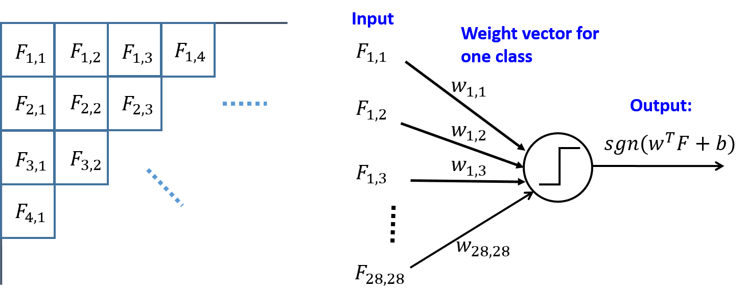
Apply the multi-class (non-differentiable) perceptron learning rule from lecture to the digit classification problem from Assignment 3. As before, the basic feature set consists of a single binary indicator feature for each pixel. Specifically, the feature F_i,j indicates the status of the (i,j)-th pixel. Its value is 1 if the pixel is foreground (no need to distinguish between the two different foreground values), and 0 if it is background. The images are of size 28*28, so there are 784 features in total. For multi-class perceptron, you need to learn a weight vector for each digit class. Each component of a weight vector corresponds to the weight of a pixel, which makes it length 784.



You should report the following:

• Training curve: overall accuracy on the training set as a function of the epoch (i.e., complete pass through the training data). It's fine to show this in table form.
• Overall accuracy on the test set.
• Confusion matrix.

To get your results, you should tune the following parameters (it is not necessary to separately report results for multiple settings, only report which options you tried and which one worked the best):

• Learning rate decay function;
• Bias vs. no bias;
• Initialization of weights (zeros vs. random);
• Ordering of training examples (fixed vs. random);
• Number of epochs.

Finally, compare the accuracies you got with perceptrons to the ones you got with Naive Bayes in Assignment 3 and discuss any interesting differences. (Your performance with perceptrons should be better than with Naive Bayes.)

Part 1.2 (for 4-unit students): Digit Classification with Nearest Neighbor

Implement a k-nearest-neighbor classifier for the digit classification task in Part 2.1. You should play around with different choices of distance or similarity function to find what works the best. In the report, please discuss your choice of distance/similarity function, and give the overall accuracy on the test set as a function of k (for some reasonable range of k). For the best choice of k, give the confusion matrix. Next, discuss the running time of your approach: how long does the nearest neighbor search take, and how does it scale with k? Finally, compare your nearest-neighbor accuracy to the accuracies you got with Naive Bayes and Perceptron. (Your best performance should be over 80%.)

Part 1 extra credit

• Incorporate the advanced features from Assignment 3 into your digit representation and see if you can get improved perceptron classification performance.
• For digits, it is possible to visualize the learned perceptron weights for each class as an image. Show some visualizations and discuss what they tell us about the model learned by the classifier -- in particular, which locations are the most important/discriminative for each digit. What do the signs of the weights tell us?
• Implement the differentiable perceptron learning rule and compare its behavior with the non-differentiable one.
• Apply any other classifier (support vector machine, decision tree, logistic regression, etc.) to digits, faces, or text. It is fine to use off-the-shelf code from an existing package (but be sure to cite your sources).

---

Part 2: Q-Learning (Pong) (for everybody)

Created by Daniel Calzada

In 1972, the game of Pong was released by Atari. Despite its simplicity, it was a ground-breaking game in its day, and it has been credited as having helped launch the video game industry. In this assignment, you will create a simple version of Pong and use Q-learning to train an agent to play the game.


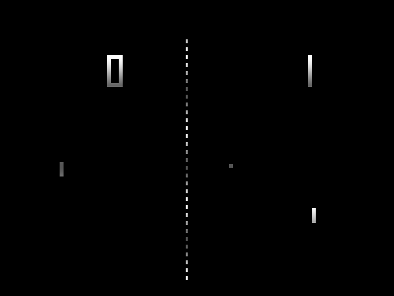
Image from Wikipedia

Setup for Single-Player Pong (for everybody)

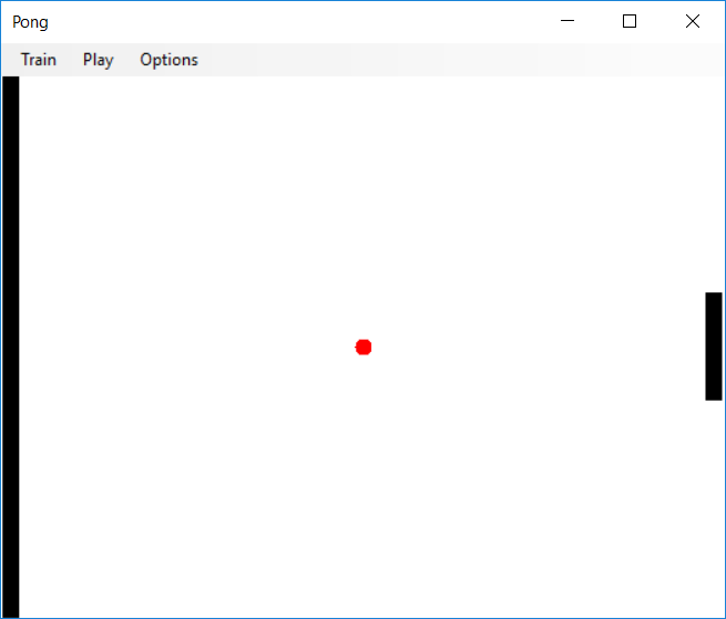
Single-player Pong

Before implementing the Q-learning algorithm, we must first write the code for the gameplay of a single-player version of Pong. If you plan on doing the 4-unit assignment, reading both parts and implementing the pong gameplay functionality with this in mind may save you time in the long-run. Since we will eventually be using Q-learning to create an AI, we must first define the Markov Decision Process (MDP):

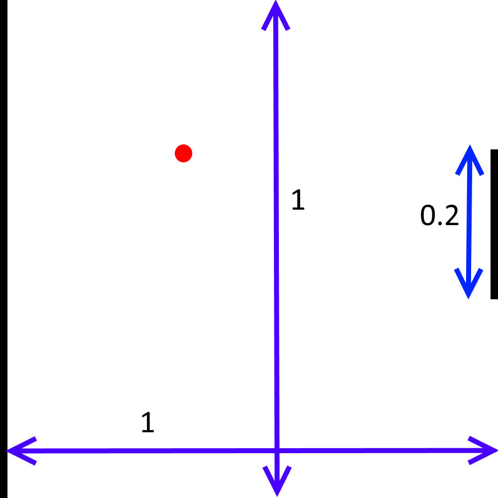
• State: A tuple (ball_x, ball_y, velocity_x, velocity_y, paddle_y).
  • ball_x and ball_y are real numbers on the interval [0,1]. The lines x=0, y=0, and y=1 are walls; the ball bounces off a wall whenever it hits. The line x=1 is defended by your paddle.
  • The absolute value of velocity_x is at least 0.03, guaranteeing that the ball is moving either left or right at a reasonable speed.
  • paddle_y represents the top of the paddle and is on the interval [0, 1 - paddle_height], where paddle_height = 0.2, as can be seen in the image above. (The x-coordinate of the paddle is always paddle_x=1, so you do not need to include this variable as part of the state definition).
• Actions: Your agent's actions are chosen from the set {nothing, paddle_y += 0.04, paddle_y -= 0.04}. In other words, your agent can either move the paddle up, down, or make it stay in the same place. If the agent tries to move the paddle too high, so that the top goes off the screen, simply assign paddle_y = 0. Likewise, if the agent tries to move any part of the paddle off the bottom of the screen, assign paddle_y = 1 - paddle_height.
• Rewards: +1 when your action results in rebounding the ball with your paddle, -1 when the ball has passed your agent's paddle, or 0 otherwise.
• Initial State: Use (0.5, 0.5, 0.03, 0.01, 0.5 - paddle_height / 2) as your initial state (see the state representation above). This represents the ball starting in the center and moving towards your agent in a downward trajectory, where the agent's paddle starts in the middle of the screen.
• Termination: Consider a state terminal if the ball's x-coordinate is greater than that of your paddle, i.e., the ball has passed your paddle and is moving away from you.

The ball is a single point, and your paddle is a line. Therefore, you don't need to worry about the ball bouncing off the ends of the paddle.

To simulate the environment at each time step, you must:

• Increment ball_x by velocity_x and ball_y by velocity_y.
• Bounce:
  • If ball_y < 0 (the ball is off the top of the screen), assign ball_y = -ball_y and velocity_y = -velocity_y.
  • If ball_y > 1 (the ball is off the bottom of the screen), let ball_y = 2 - ball_y and velocity_y = -velocity_y.
  • If ball_x < 0 (the ball is off the left edge of the screen), assign ball_x = -ball_x and velocity_x = -velocity_x.
  • If moving the ball to the new coordinates resulted in the ball bouncing off the paddle, handle the ball's bounce by assigning ball_x = 2 * paddle_x - ball_x. Furthermore, when the ball bounces off a paddle, randomize the velocities slightly by using the equation velocity_x = -velocity_x + U and velocity_y = velocity_y + V, where U is chosen uniformly on [-0.015, 0.015] and V is chosen uniformly on [-0.03, 0.03]. As specified above, make sure that all |velocity_x| > 0.03.
    
    Note: In rare circumstances, either of the velocities may increase above 1. In these cases, after applying the bounce equations given above, the ball may still be out of bounds. If this poses a problem for your implementation, feel free to impose the restriction that |velocity_x| < 1 and |velocity_y| < 1.

Because this state space is continuous, to allow for it to be learned with Q-learning, we need to be able to convert the continuous state space into a discrete, finite state space. To do this, please follow the instructions below. Note that the constants may be different for the next part of the assignment, so it would be wise to define these as constants in a separate part of your code so you can change them easily.

• Treat the entire board as a 12x12 grid, and let two states be considered the same if the ball lies within the same cell in this table. Therefore there are 144 possible ball locations.
• Discretize the X-velocity of the ball to have only two possible values: +1 or -1 (the exact value does not matter, only the sign).
• Discretize the Y-velocity of the ball to have only three possible values: +1, 0, or -1. It should map to Zero if |velocity_y| < 0.015.
• Finally, to convert your paddle's location into a discrete value, use the following equation: discrete_paddle = floor(12 * paddle_y / (1 - paddle_height)). In cases where paddle_y = 1 - paddle_height, set discrete_paddle = 11. As can be seen, this discrete paddle location can take on 12 possible values.
• Add one special state for all cases when the ball has passed your paddle (ball_x > 1). This special state needn't differentiate among any of the other variables listed above, i.e., as long as ball_x > 1, the game will always be in this state, regardless of the ball's velocity or the paddle's location. This is the only state with a reward of -1.
• Therefore, the total size of the state space for this problem is (144)(2)(3)(12)+1 = 10369.

Part 2.1: Single-Player Pong (for everybody)

Untrained (random) agent	Trained agent

In this part of the assignment, you will create a single-player pong game, where the agent must learn how to bounce the ball off the paddle as many times as possible. In order to do this, you must use Q-learning. Implement the Q-learning algorithm and train it on the MDP outlined above. Train it for as long as you deem necessary, counting the average number of times your agent can get the ball to bounce off its paddle before missing the ball. Your agent should at least be able to rebound the ball at least nine consecutive times before missing it, although your results may be significantly better than this (as high as 12-14). In order to achieve an optimal policy, you will need to adjust the learning rate, α, the discount factor, γ, and the settings that you use to trade off exploration vs. exploitation.

In your report, please include the values of α, γ, and any parameters for your exploration settings that you used, and discuss how you obtained these values. What changes happen in the game when you adjust any of these variables? How many games does your agent need to simulate before it learns an optimal policy? After your Q-learning seems to have converged to a good policy, run your algorithm on a large number of test games (≥1000) and report the average number of times the ball bounces off your paddle before the ball escapes past the paddle (you may continue learning during these test games, or you may disable learning).

In addition to discussing these things, try adjusting the discretization settings that were defined above, for example, changing the resolution of the grid to something besides 12x12, or changing the set of possible velocities of the ball. If you think it would be beneficial, you may also change the reward model to provide more informative feedback to the agent (as long as it does not trivialize the assignment). Try to find modifications that allow the agent to learn a better policy than the one you found before. In your report, describe the changes you made and the new number of times the agent was able to rebound the ball (it should be greater than what you found before). What effect did this have on the time it takes to train your agent? Include any other interesting observations.

Tips

• To get a better understanding of the Q learning algorithm, read section 21.3 of the textbook.
• Initially, all the Q value estimates should be 0.
• For choosing a discount factor, try to make sure that the reward from the previous rebound has a limited effect on the next rebound. In other words, choose your discount factor so that as the ball is approaching your paddle again, the reward from the previous hit has been mostly discounted.
• The learning rate should decay as C/(C+N(s,a)), where N(s,a) is the number of times you have seen the given the state-action pair and C is a constant that you must choose.
• To learn a good policy, you need on the order of 100K games, which should take just a few minutes in a reasonable implementation.

Part 2.2: Two-Player Pong (for 4-unit students, extra credit for 3-unit students)

Left: hard-coded agent; right: trained agent


Now that you have implemented a version of Pong for a single-player, create a second player on the left of your screen, against whom your AI agent can play. The second player's policy will be hard-coded. Have your second player move always in the direction of the ball, so that the center of the paddle is closer to the y-coordinate of the ball (in this way, the hard-coded AI will 'track' the ball as it bounces up and down). However, the hard-coded opponent's paddle can only move half as fast as the your agent's paddle. Formally, the opponent's action is chosen from {nothing, paddle_y += 0.02, paddle_y -= 0.02}. The opponent's paddle's height is the same as your agent's.

Here are some questions and things for you to consider as you adjust your MDP, Q-learning parameters, and implementation. Please include your responses in your report.

• What changes do you need to make to your MDP (state space, actions, and reward model), if any? Would there be any negative side-effects of doing this?
• Describe any other changes you needed to make to your implementation.
• When your agent has been fully trained, what percentage of the time can it defeat the hard-coded agent (i.e. make the opponent miss the ball)? You should be able to defeat the hard-coded agent in at least 75% of the games you run, although it could be much better.

Part 2 Extra Credit

• Create a graphical representation of your Pong game. A GUI would be preferable, but a text-based console implementation is also acceptable, as long as the text characters are redrawn in place (the image of the playing court does not move around on the screen).
• If you created either a GUI or a console-based implementation, allow for a human to play against the AI. Are you able to defeat it? What are its strengths and weaknesses? Describe your discoveries.
• Create and include an animation of your agent playing the game.
• Add more complexity to the game (power-ups, put the table on a slant to make the ball gravitate to one side, and so on), and observe and describe how your Q-learning agent adjusts to the changes in the environment, finding a new optimal policy. Keep in mind the size of your state space---making a handful of small changes may exponentially increase this.

---

Report Checklist

Part 1:

1. (for everybody): Discuss your implementation of perceptron classifier and parameter settings. Show your training curve, overall accuracy, and confusion matrix. Compare the accuracy to Naive Bayes method from Assignment 3.
2. (for four-unit students): Discuss your distance/similarity function, give the overall test set accuracy as a function of k, give confusion matrix for best k. Discuss running time, and compare your accuracy to Naive Bayes and perceptron.

Part 2.1: (for everybody)

1. Report and justify your choices for α, γ, exploration function, and any subordinate parameters. How many games does your agent need to simulate before it learns a good policy?
2. Use α, γ, and exploration parameters that you believe to be the best. After training has converged, run your algorithm on a large number of test games (≥1000) and report the average number of times per game that the ball bounces off your paddle before the ball escapes past the paddle.
4. Describe how you changed the MDP and/or the constants used to discretize the continuous state space you made. Discuss what effect, if any, this had on the time it takes to train your agent, and any other interesting observations. For at least one set of changed game state or action variables, run a converged algorithm on at least 1000 test games, and report the new number of times the agent was able to rebound the ball.

Part 2.2: (for 4-unit students)

1. Describe the changes you made to your MDP (state space, actions, and reward model), if any, and include any negative side-effects you encountered after doing this.
2. Describe any other changes you needed to make to your implementation.
3. Report the percentage of the time your fully-trained AI can defeat the hard-coded agent?

Submission Instructions

As usual, one designated person from the group will need to submit on Compass 2g by the deadline. Three-unit students must upload under Assignment 4 (three units) and four-unit students must upload under Assignment 4 (four units). Each submission must consist of the following two attachments:

1. A report in PDF format. As usual, the report should briefly describe your implemented solution and fully answer all the questions posed above. Remember: you will not get credit for any solutions you have obtained, but not included in the report.

   All group reports need to include a brief statement of individual contribution, i.e., which group member was responsible for which parts of the solution and submitted material.
   
   The name of the report file should be lastname_firstname_assignment4.pdf. Don't forget to include the names and NetIDs of all group members and the number of credit units at the top of the report.

2. Your source code compressed to a single ZIP file. The code should be well commented, and it should be easy to see the correspondence between what's in the code and what's in the report. You don't need to include executables or various supporting files (e.g., utility libraries) whose content is irrelevant to the assignment. If we find it necessary to run your code in order to evaluate your solution, we will get in touch with you.
   
   The name of the code archive should be lastname_firstname_assignment4.zip.

Multiple attempts will be allowed but in most circumstances, only the last submission will be graded. We reserve the right to take off points for not following directions.

Late policy: For every day that your assignment is late, your score gets multiplied by 0.75. The penalty gets saturated after four days, that is, you can still get up to about 32% of the original points by turning in the assignment at all. If you have a compelling reason for not being able to submit the assignment on time and would like to make a special arrangement, you must send me email at least four days before the due date (any genuine emergency situations will be handled on an individual basis).

Extra credit:

• We reserve the right to give bonus points for any advanced exploration or especially challenging or creative solutions that you implement. Three-unit students always get extra credit for submitting solutions to four-unit problems. If you submit any work for bonus points, be sure it is clearly indicated in your report.

Statement of individual contribution:

• All group reports need to include a brief summary of which group member was responsible for which parts of the solution and submitted material. We reserve the right to contact group members individually to verify this information.

WARNING: You will not get credit for any solutions that you have obtained, but not included in your report! For example, if your code prints out path cost and number of nodes expanded on each input, but you do not put down the actual numbers in your report, or if you include pictures/files of your output solutions in the zip file but not in your PDF. The only exception is animated paths (videos or animated gifs).

Be sure to also refer to course policies on academic integrity, etc.