CS 543 Fall 2021
Assignment 4: Deep Convolutional Neural Networks
Due date: Thursday, December 2, 11:59:59PM
The goal of this assignment is to get hands-on experience designing and training deep convolutional neural networks using PyTorch. Starting from a baseline architecture we provided, you will design an improved deep net architecture to classify (small) images into 100 categories. You will evaluate the performance of your architecture by uploading your predictions to two Kaggle competitions for Part1 and Part2 respectively and submit your code and report describing your implementation choices to Compass2g.
Table of contents:
- PyTorch
- Google Colab Setup
- Part 1: Improving BaseNet on CIFAR100
- Part 2: Transfer Learning
- Extra Credit
- Submission Checklist
Deep Learning Framework: PyTorch
In this assignment you will use PyTorch, which is currently one of the most popular deep learning frameworks and is very easy to pick up. It has a lot of tutorials and an active community answering questions on its discussion forums. Part 1 has been adapted from a PyTorch tutorial on the CIFAR-10 dataset. Part 2 has been adapted from the PyTorch Transfer Learning tutorial.
Google Colab Setup
You will be using Google Colab, a free environment to run your experiments. Here are instructions on how to get started:
- Open Colab, click on 'File' in the top left corner and select upload 'New Python 3 Notebook'. Upload this notebook.
- In your Google Drive, create a new folder titled 'MP4'. This is the folder that will be mounted to Colab. All outputs generated by Colab Notebook will be saved here.
- Within the folder, create a subfolder called 'data'. Visit kaggle pages for Part1 and Part2 and click on "Download All". Upload both the zip files to the "data" folder on Google Drive.
- Follow the instructions in the notebook to finish the setup.
- Based on the description in Overview section, comments indicating where changes should be made have been included in this file.
Part 1: Improving BaseNet on CIFAR100
Dataset
For this part of the assignment, you will be working with the CIFAR100
dataset (already loaded above). This dataset consists of 60K 32x32
color images from 100 classes, with 600 images per class. There are 50K
training images and 10K test images. The images in CIFAR100 are of size
3x32x32, i.e. 3-channel color images of 32x32 pixels.
We have modified the standard dataset to create the
CIFAR100_CS543 dataset which consists of 45K training images (450 of
each class), 5K validation images (50 of each class), and 10K test
images (100 of each class). The train and val datasets have labels while
all the labels in the test set are set to 0. You can tune your model on
the validation set and obtain your performance on the test set by
uploading a CSV file to this Kaggle competition. Note that you are
limited to 5 submissions a day, so try to tune your model before
uploading CSV files. Also, you must make at least one submission for
your final system for full credit. The best performance will be
considered.
BaseNet
We created a BaseNet that you can run and get a baseline accuracy (~23% on the test set). The starter code for this is in the BaseNet class. It uses the following neural network layers:
- Convolutional, i.e. nn.Conv2d
- Pooling, e.g. nn.MaxPool2d
- Fully-connected (linear), i.e. nn.Linear
- Non-linear activations, e.g. nn.ReLU
- Normalization, e.g. nn.batchnorm2d
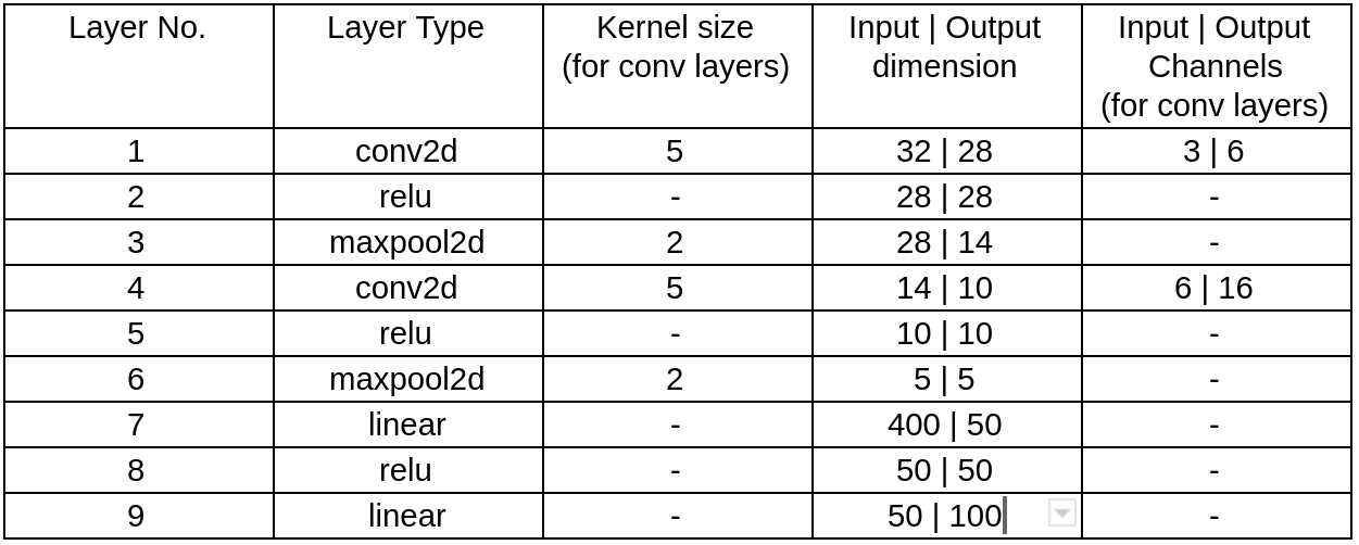
Your goal is to edit the BaseNet class or make new classes for devising a more accurate deep net architecture. In your report, you will need to include a table similar to the one above to illustrate your final network.
Before you design your own architecture, you should start by getting familiar with the BaseNet architecture already provided, the meaning of hyper-parameters and the function of each layer. This tutorial by PyTorch is helpful for gearing up on using deep nets. Also, this lecture on CNN by Andrej Karpathy is a good resource for anyone starting with deep nets. It talks about architectural choices, output dimension of conv layers based on layer parameters, and regularization methods. For more information on learning rates and preventing overfitting, this lecture is a good additional read.
Improve your model
As stated above, your goal is to create an improved deep net by
making judicious architecture and implementation choices. A good
combination of choices can get your accuracy close to 50%. A reasonable
submission with more than 40% accuracy will be given full credit. For
improving the network, you should consider all of the following.
1. Data normalization. Normalizing input data makes training easier and more robust. Similar to normalized epipolar geometry estimation, data in this case too could be made zero mean and fixed standard deviation (sigma=1 is the to-go choice). Use transforms.Normalize() with the right parameters to make the data well conditioned (zero mean, std dev=1) for improved training. After your edits, make sure that test_transform has the same data normalization parameters as train_transform.
2. Data augmentation. Try using transforms.RandomCrop() and/or transforms.RandomHorizontalFlip() to augment training data. You shouldn't have any data augmentation in test_transform (val or test data is never augmented). If you need a better understanding, try reading through PyTorch tutorial on transforms.
3. Deeper network. Following the guidelines laid out by this lecture on CNN, experiment by adding more convolutional and fully connected layers. Add more conv layers with increasing output channels and also add more linear (fc) layers. Do not put a maxpool layer after every conv layer in your deeper network as it leads to too much loss of information.
4. Normalization layers. Normalization layers help reduce overfitting and improve training of the model. Pytorch's normalization layers are an easy way of incorporating them in your model. Add normalization layers after conv layers (nn.BatchNorm2d). Add normalization layers after linear layers (nn.BatchNorm1d) and experiment with inserting them before or after ReLU/Maxpool layers.
5. Early stopping. After how many epochs to stop training? This answer on stackexhange is a good summary of using train-val-test splits to reduce overfitting. This blog is also a good reference for early stopping. Remember, you should never use the test-set in anything but the final evaluation. Seeing the train loss and validation accuracy plot, decide for how many epochs to train your model. Not too many (as that leads to overfitting) and not too few (else your model hasn't learnt enough).
Finally, there are a lot of approaches to improve a model beyond what we listed above. For possible extra credit, feel free to try out your own ideas, or interesting ML/CV approaches you read about. Since Colab makes only limited computational resources available, we encourage you to rationally limit training time and model size.
Kaggle Submission
Running Part 1 in the Colab notebook creates a plot.png and submission_netid.csv file in the MP4 folder in your Google Drive. The plot needs to go into your report and the csv file needs to be uploaded to Kaggle.Tips
- Do not lift existing code or torchvision models.
- All edits to BaseNet which lead to a significant accuracy improvement must be listed in the report. Try also to support this explanation by adding an entry in the ablation study. We understand running experiments for each change might get cumbersome if you are trying a lot of things. So use your judgment to decide what are the most important factors to getting improved performance and documenting how you evolved your model.
Part 2: Transfer Learning
In this part, you will fine-tune a ResNet model pre-trained on ImageNet for classifying the Caltech-UCSD Birds dataset. This dataset consists of 200 categories of birds, with 2400 images in train, 600 in validation and 3033 images in test. Follow the instructions in the notebook and complete the sections marked #TODO. Submit the generated CSV file in the part-2 competition page mentioned above to know the test accuracy. Like part-1, submissions are limited to 5 per day. Without changing the given hyperparameters, you should achieve a test accuracy of 5.86%. With slight tweaks to the hyperparameters and a good choice of transforms, you should be able to get a test accuracy close to 51%. A reasonable submission with more than 45% accuracy will be given full credit.Experiment with the following:
- Vary the hyperparameters based on how your model performs on
train in the current setting. You can increase the number of epochs up
to 30.
- Augment the data similarly to Part 1.
- ResNet as a fixed feature extractor. The current
setting in the provided notebook allows you to use the ResNet
pre-trained on ImageNet as a fixed feature extractor. We freeze the
weights for all of the network except that of the final fully connected
layer. This last fully connected layer is replaced with a new one with
random weights and only this layer is trained.
- Fine-tuning the ResNet. To fine-tune the entire ResNet, instead of only training the final layer, set the parameter RESNET_LAST_ONLY to False.
- Try different learning rates in the following range: 0.0001 to 0.01.
- If you're feeling adventurous, try loading other pre-trained networks avaliable in Pytorch.
A few useful resources:
- This Kaggle tutorial is a helpful resource on using pre-trained models in pytorch.
- This post explains how to fine-tune a model in pytorch.
- https://arxiv.org/abs/1403.6382 - trains SVMs on features from ImageNet-trained ConvNet and reports several state of the art results.
- https://arxiv.org/abs/1310.1531 - reports similar findings.
- https://arxiv.org/abs/1411.1792 - studies transfer learning in detail.
Extra Credit
For both Parts 1 and 2, extra credit can be any extensions to the model or advanced learning tricks, beyond the basics described here. One suggestion is using an adaptive learning rate.Submission Checklist
- Part 1:
- CSV file of your predicted test labels needs to be uploaded to Kaggle. Your performance will not directly affect your grade unless it is below our threshold of 40%.
- The report should include the following:
- The name under which you submitted on Kaggle.
- Best accuracy (should match your accuracy on Kaggle).
- Table defining your final architecture similar to the image above.
- Factors which helped improve your model performance. Explain each factor in 2-3 lines.
- Final architecture’s plot for training loss and validation accuracy. This would have been auto-generated by the notebook.
- Ablation study to validate the above choices, i.e., a comparison of performance for two variants of a model, one with and one without a certain feature or implementation choice.
- Explanation of any extra credit features if attempted.
- Part 2:
- Report the train and test accuracy achieved by using the ResNet as a fixed feature extractor vs. fine-tuning the whole network.
- Report the hyperparameter settings you used and explain how you came up with these settings(batch_size, learning_rate, resnet_last_only, num_epochs).
- Explain the transformations you used on the train set. Discuss how including/excluding each of them made a difference in the accuracy.
Instructions for turning in the assignment
You must upload the following files to Compass 2g:- Your Colab notebook. The filename should be netid_mp4.ipynb. In the notebook, make sure the hyperparameters set in both Parts 1 and 2 achieve the best results you report.
- A single report for both parts in PDF format. The filename should be netid_mp4_report.pdf.
Don't forget to hit "Submit" on Compass after uploading your files, otherwise we will not receive your submission.
Please refer to course policies on using external sources, late submission, etc.