Spring 2016 CS543/ECE549

Extra Credit Assignment

Due date: Wednesday, April 27, 11:59:59PM -- No late submissions accepted!

• Affine factorization
• Single-view geometry
• Binocular stereo
• Instructions for turning in the assignment

The goal of this part of the assignment is to implement the Tomasi and Kanade affine structure from motion method as described in this lecture. You will be working with Carlo Tomasi's 101-frame hotel sequence:

Download the data file, including all the 101 images and a measurement matrix consisting of 215 points visible in each of the 101 frames (see readme file inside archive for details).

1. Load the data matrix and normalize the point coordinates by translating them to the mean of the points in each view (see lecture for details).
   
   
2. Apply SVD to the 2M x N data matrix to express it as D = U * W * V' where U is a 2Mx3 matrix, W is a 3x3 matrix of the top three singular values, and V is a Nx3 matrix. Derive structure and motion matrices from the SVD as explained in the lecture.
   
   
3. Use plot3 to display the 3D structure (in your report, you may want to include snapshots from several viewpoints to show the structure clearly). Discuss whether or not the reconstruction has an ambiguity.
   
   
4. Display three frames with both the observed feature points and the estimated projected 3D points overlayed. Report your total residual (sum of squared Euclidean distances, in pixels, between the observed and the reprojected features) over all the frames, and plot the per-frame residual as a function of the frame number.

Part 1 Extra-Extra Credit

• Attempt to eliminate the affine ambiguity using the method described in the lecture.
  
  
• Incorporate incomplete point tracks (i.e., points that are not visible in every frame) into the reconstruction. Use the tracks from this file.
  
  
• Create a textured 3D model of the reconstructed points. For example, you can compute a Delaunay triangulation of the points in 2D, then lift that mesh structure to 3D, and texture it using the images.

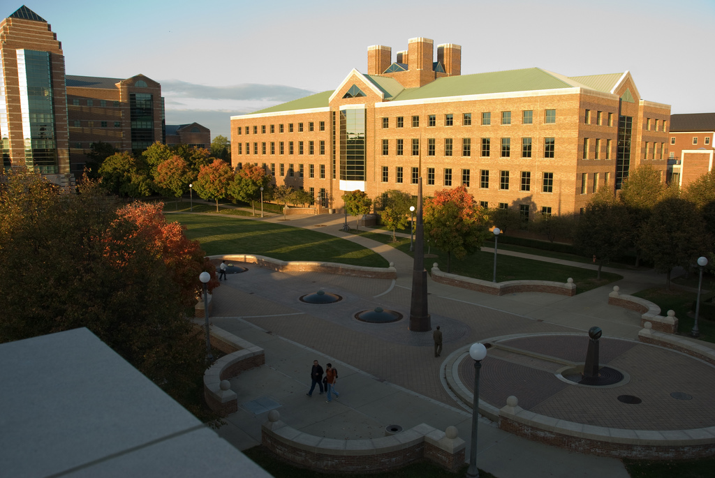
Part 2: Single-View Geometry

Adapted from Derek Hoiem by Tom Paine

1. For the above image of the north quad, estimate the three major orthogonal vanishing points. Use at least three manually selected lines to solve for each vanishing point. This MATLAB code provides an interface for selecting and drawing the lines, but the code for computing the vanishing point needs to be inserted. For details on estimating vanishing points, see Derek Hoiem's book chapter (section 4). You should also refer to this chapter and the single-view metrology lecture for details on the subsequent steps. In your report, you should:
   • Plot the VPs and the lines used to estimate them on the image plane using the provided code.
   • Specify the VP pixel coordinates.
   • Plot the ground horizon line and specify its parameters in the form a * x + b * y + c = 0. Normalize the parameters so that: a^2 + b^2 = 1.
   
   
2. Using the fact that the vanishing directions are orthogonal, solve for the focal length and optical center (principal point) of the camera. Show all your work.
   
   
3. Compute the rotation matrix for the camera, setting the vertical vanishing point as the Y-direction, the right-most vanishing point as the X-direction, and the left-most vanishing point as the Z-direction.
   
   
4. Estimate the heights of (a) the CSL building, (b) the spike statue, and (c) the lamp posts assuming that the person nearest to the spike is 5ft 6in tall. In the report, show all the lines and measurements used to perform the calculation. How do the answers change if you assume the person is 6ft tall?

Part 2 Extra-Extra Credit

• Perform additional measurements on the image: which of the people visible are the tallest? What are the heights of the windows? etc.
  
  
• Compute and display rectified views of the ground plane and the facades of the CSL building.
  
  
• Attempt to fit lines to the image and estimate vanishing points automatically either using your own code or code downloaded from the web.
  
  
• Find or take other images with three prominently visible orthogonal vanishing points and demonstrate varions measurements on those images.

Follow the basic outline given in this lecture: pick a window around each pixel in the first (reference) image, and then search the corresponding scanline in the second image for a matching window. The output should be a disparity map with respect to the first view (use this ground truth map for qualitative reference). You should experiment with the following settings and parameters:

• Search window size: show disparity maps for several window sizes and discuss which window size works the best (or what are the tradeoffs between using different window sizes). How does the running time depend on window size?
  
  
• Disparity range: what is the range of the scanline in the second image that should be traversed in order to find a match for a given location in the first image? Examine the stereo pair to determine what is the maximum disparity value that makes sense, where to start the search on the scanline, and which direction to search in. Report which settings you ended up using.
  
  
• Matching function: try sum of squared differences (SSD) and normalized correlation. Discuss in your report whether there is any difference between using these two functions, both in terms of quality of the results and in terms of running time.

Part 3 Extra-Extra Credit

• Convert your disparity map to a depth map and attempt to visualize the depth map in 3D. Just pretend that all projection rays are parallel, and try to "guess" the depth scaling constant. Experiment with displaying a 3D point cloud, or computing a Delaunay triangulation of that point cloud.
  
  
• Find additional rectified stereo pairs on the Web and show the results of your algorithm on these pairs.
  
  
• Find non-rectified stereo pairs and rectification code on the Web and apply your algorithm to this data.
  
  
• Implement multiple-baseline stereo as described in this lecture (see paper by Okutomi and Kanade). Use this data.
  
  
• Try to incorporate non-local constraints (smoothness, uniqueness, ordering) into your algorithm. You can come up with simple heuristic ways of incorporating these constraints, or try to implement some of the more advanced methods discussed in the course (dynamic programming, graph cuts). For this part, it is also fine to find code on the web.