CS440/ECE448 Fall 2017

Assignment 3: Naive Bayes Classification

Due: Monday, November 27th, 11:59:59PM

Contents

• Part 1: Digit classification
  • Part 1.1 (for everybody): Single pixels as features
  • Part 1.2 (for four-credit students): Pixel groups as features
• Part 2: Audio classification
  • Part 2.1 (for everybody): Hebrew "Yes/No" Classification
  • Part 2.2 (for four-credit students): Audio Digit Classification
• Report checklist
• Submission instructions

Part 1: Digit classification

Part 1.1 (for everybody): Single pixels as features

• Features: The basic feature set consists of a single binary indicator feature for each pixel. Specifically, the feature F_ij indicates the status of the (i,j)-th pixel. Its value is 1 if the pixel is foreground (no need to distinguish between the two different foreground values), and 0 if it is background. The images are of size 28*28, so there are 784 features in total.

• Training: The goal of the training stage is to estimate the likelihoods P(F_ij | class) for every pixel location (i,j) and for every digit class from 0 to 9. The likelihood estimate is defined as
  
  P(F_ij = f | class) = (# of times pixel (i,j) has value f in training examples from this class) / (Total # of training examples from this class)
  
  In addition, as discussed in the lecture, you have to smooth the likelihoods to ensure that there are no zero counts. Laplace smoothing is a very simple method that increases the observation count of every value f by some constant k. This corresponds to adding k to the numerator above, and k*V to the denominator (where V is the number of possible values the feature can take on). The higher the value of k, the stronger the smoothing. Experiment with different values of k (say, from 0.1 to 10) and find the one that gives the highest classification accuracy.
  
  You should also estimate the priors P(class) by the empirical frequencies of different classes in the training set.
   
• Testing: You will perform maximum a posteriori (MAP) classification of test digits according to the learned Naive Bayes model. Suppose a test image has feature values f_1,1, f_1,2, ... , f_28,28. According to this model, the posterior probability (up to scale) of each class given the digit is given by
  
  P(class) ⋅ P(f_1,1 | class) ⋅ P(f_1,2 | class) ⋅ ... ⋅ P(f_28,28 | class)
  
  Note that in order to avoid underflow, it is standard to work with the log of the above quantity:
  
  log P(class) + log P(f_1,1 | class) + log P(f_1,2 | class) + ... + log P(f_28,28 | class)
  
  After you compute the above decision function values for all ten classes for every test image, you will use them for MAP classification.
   
• Evaluation: Use the true class labels of the test images from the testlabels file to check the correctness of the estimated label for each test digit. Report your performance in terms of the classification rate for each digit (percentage of all test images of a given digit correctly classified). Also report your confusion matrix. This is a 10x10 matrix whose entry in row r and column c is the percentage of test images from class r that are classified as class c. In addition, for each digit class, show the test examples from that class that have the highest and the lowest posterior probabilities according to your classifier. You can think of these as the most and least "prototypical" instances of each digit class (and the least "prototypical" one is probably misclassified).
  
  Important: The ground truth labels of test images should be used only to evaluate classification accuracy. They should not be used in any way during the decision process.
  
  Tip: You should be able to achieve at least 70% accuracy on the test set. One "warning sign" that you have a bug in your implementation is if some digit gets 100% or 0% classification accuracy (that is, your system either labels all the test images as the same class, or never wants to label any test images as some particular class).
   
• Odds ratios: When using classifiers in real domains, it is important to be able to inspect what they have learned. One way to inspect a naive Bayes model is to look at the most likely features for a given label. Another tool for understanding the parameters is to look at odds ratios. For each pixel feature F_ij and pair of classes c₁, c₂, the odds ratio is defined as
  
  odds(F_ij=1, c₁, c₂) = P(F_ij=1 | c₁) / P(F_ij=1 | c₂).
  
  This ratio will be greater than one for features which cause belief in c₁ to increase over the belief in c₂. The features that have the greatest impact on classification are those with both a high probability (because they appear often in the data) and a high odds ratio (because they strongly bias one label versus another).
  
  Take four pairs of digits that have the highest confusion rates according to your confusion matrix, and for each pair, display the maps of feature likelihoods for both classes as well as the odds ratio for the two classes. For example, the figure below shows the log likelihood maps for 1 (left), 8 (center), and the log odds ratio for 1 over 8 (right):
  
  
  
  If you cannot do a graphical display like the one above, you can display the maps in ASCII format using some coding scheme of your choice. For example, for the odds ratio map, you can use '+' to denote features with positive log odds, ' ' for features with log odds close to 1, and '-' for features with negative log odds.

Part 1.2 (for four-credit students): Pixel groups as features

Credit: Yanglei Song

Instead of each feature corresponding to a single pixel, we can form features from groups of adjacent pixels. We can view this as a relaxation of the Naive Bayes assumption that allows us to have a more accurate model of the dependencies between the individual random variables. Specifically, consider a 2*2 square of pixels with top left coordinate i,j and define a feature G_i,j that corresponds to the ordered tuple of the four pixel values. For example, in the figure below, we have

G_1,1 = (F_1,1, F_1,2, F_2,1, F_2,2).



(The exact ordering of the four pixel values is not important as long as it's consistent throughout your implementation.) Clearly, this feature can have 16 discrete values. The 2*2 squares can be disjoint (left side of figure) or overlapping (right side of figure). In the case of disjoint squares, there are 14 * 14 = 196 features; in the case of overlapping squares, there are 27 * 27 = 729 features.

We can generalize the above examples of 2*2 features to define features corresponding to n*m disjoint or overlapping pixel patches. An n*m feature will have 2^n*m distinct values, and as many entries in the conditional probability table for each class. Laplace smoothing applies to these features analogously as to the single pixel features.

In this part, you should build Naive Bayes classifiers for feature sets of n*m disjoint/overlapping pixel patches and report the following:

• Test set accuracies for disjoint patches of size 2*2, 2*4, 4*2, 4*4.
• Test set accuracies for overlapping patches of size 2*2, 2*4, 4*2, 4*4, 2*3, 3*2, 3*3.
• Discussion of the trends you have observed for the different feature sets (including single pixels), in particular, why certain features work better than others for this task.
• Brief discussion of running time for training and testing for the different feature sets (which ones are faster and why, and how does the running time scale with feature set size).

Part 1 Extra Credit

• Experiment with yet more features to improve the accuracy of the Naive Bayes model. For example, instead of using binary pixel values, implement ternary features. Alternatively, try using features that check to see if there is a horizontal line of three consecutive foreground pixels, or a vertical or diagonal line.
   
• Apply your Naive Bayes classifier with various features to this face data. It is in a similar format to that of the digit data, and contains training and test images and binary labels, where 0 corresponds to 'non-face' and 1 corresponds to 'face'. The images themselves are higher-resolution than the digit images, and each pixel value is either '#', corresponding to an edge being found at that location, or ' ', corresponding to a non-edge pixel.

Part 2: Audio Classification

Created by Ryley Higa and Huozhi Zhou based on Audiovisual Person Identification

Part 2.1: For everybody

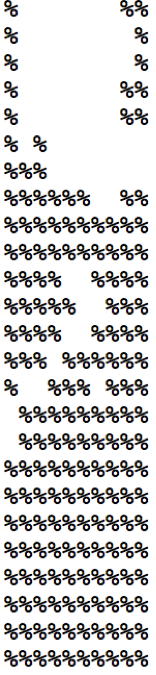
The goal of this part is to apply Naive Bayes classifiers to solve basic binary classification problems in the area of audio signal processing. The specific task is to distinguish between the Hebrew words of "yes" and "no". The feature representation is in the form of a binarized text image of a spectrogram, where the horizontal direction is the time axis and the vertical direction is the frequency axis. Blank means "high energy" and "%" means "low energy." Below, we show the original image of a spectrogram of eight successive yes/no utterances, with an example of a single binarized utterance to the right:

   

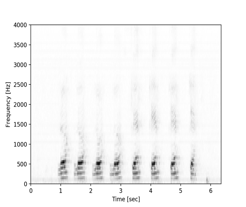
You can find a zip file with training and test data here. In each file, each individual spectrogram is 25 by 10 characters, and different spectrograms are separated by three blank lines.

Model: For this dataset, you will build a Naive Bayes classifier using the model (called a Bernoulli model) in which every spectrogram is described by 250 binary variables W_(1,1), ... , W_{(25, 10)}, and W_{(i, j)} = 1 if the ij-th block of the spectrogram has high energy and and 0 otherwise. You can estimate the likelihoods P(W_{(i, j)} = 1 | class) as the proportion of the training data from that class that has high energy at the corresponding block. Be sure to use Laplace smoothing and estimate the prior distributions of class labels.

Testing: Similar to part 1, you need to perform maximum a posteriori (MAP) classification of "yes" or "no" according to the learned model. Similar to part 1, you assume that each features are conditionally independent given the class and compute the log-likelihood to avoid underflow.

Report: In your report, briefly discuss your implementation especially the choice of Laplace smoothing constant. Give the confusion matrix for the "yes" and "no" classes.

Part 2.2: For four-credit students

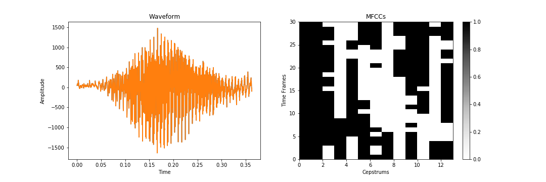
For part 2.2, your task is to classify audio digits 1-5 spoken by four different speakers. If we examined the waveform of the each spoken digit directly, it would be extremely difficult to distinguish the digit in the recording with a simple Bayesian classifier. In many audio applications, we may need more sophisticated features than the raw time series. Mel-frequency cepstrum coefficients (MFCCs) represent the short-term power spectrum of sound and are better features for speech recognition. You can find more background information on MFCCs here. For this part, you are provided with the binarized MFCCs for spoken digits 1-5. The data consists of 60 training recordings and 40 testing recordings each of which have been preprocessed. Each audio recording in the dataset is clipped or extended to 0.35-0.4 seconds, transformed into the Mel-frequency domain, and then binarized to 1 or 0 if the coefficient is above a determined threshold. From the binarized MFCCs, you should be able to correctly classify the digits spoken in each audio clip with greater than 80% overall accuracy using a Bernoulli Naive Bayes classifier.

The dataset can be found here.

Each recording in the datafile is represented as a 30 by 13 text-based spectrogram where the x-axis repesents cepstrums, the y-axis represents time frames, '%' indicates a region of low energy (0), and white spaces indicate a region of high energy (1) similiar to the text figure in part 2.1. Each spectrogram is separated by three completely blank lines. Please do not include the three blank lines as features in any of your estimates.

In your report, you should give the the overall accuracy and confusion matrix.

Extra Credit for Part 2

• Train the Part 2.1 classifier using an unsegmented version of the same data. In this archive, each training file represents a random sequence of 8 yes's or no's. The sequence is encoded in the filename, with 1 for yes and 0 for no. You need to figure out how to divide the training data into individual words (25 by 10 characters) in order to estimate the model parameters. For testing, the archive provides 50 individual binarized text images of spectrograms for both "yes" and "no".
• Classify either the yes-no corpus or the digits corpus using any alternative method not covered in class, such as Fisher's linear discriminant analysis.
• For the yes-no corpus, try classifying each test image by first computing the average column: that is, average together the 10 consecutive columns that form each image, in order to compute a 25-dimensional vector. Now, each of those 25 features can take on any one of 11 possible values (0, 1/10, 2/10, 3/10, ... , 1). Create a Naive Bayes classifier for this feature set, using appropriate settings for Laplace smoothing. Note: your accuracy will probably not be as good for this setting as for the baseline setting, but your computational complexity should be lower.

Report Checklist

Part 1:

1. For everybody:

• Briefly discuss your implementation, especially the choice of the smoothing constant.
• Report classification rate for each digit and confusion matrix.
• For each digit, show the test examples from that class that have the highest and lowest posterior probabilities according to your classifier.
• Take four pairs of digits that have the highest confusion rates, and for each pair, display feature likelihoods and odds ratio.

2. For four-credit students:

• Report test set accuracies for disjoint patches of size 2*2, 2*4, 4*2, 4*4, and for overlapping patches of size 2*2, 2*4, 4*2, 4*4, 2*3, 3*2, 3*3.
• Discuss trends for the different feature sets.
• Discuss training and testing running time for different feature sets.

Part 2:

1. For everybody: Discuss the implementation and show the confusion matrix for "yes" and "no" classes.
2. For four-credit students: Discuss the implementation, give the overall accuracy, and the confusion matrix.

Extra credit:

• We reserve the right to give bonus points for any advanced exploration or especially challenging or creative solutions that you implement. Three-credit students always get extra credit for submitting solutions to four-credit problems (at 50% discount). If you submit any work for bonus points, be sure it is clearly indicated in your report.

Statement of individual contribution:

• All group reports need to include a brief summary of which group member was responsible for which parts of the solution and submitted material. We reserve the right to contact group members individually to verify this information.

WARNING: You will not get credit for any solutions that you have obtained, but not included in your report! For example, if your code prints out path cost and number of nodes expanded on each input, but you do not put down the actual numbers in your report, or if you include pictures/files of your output solutions in the zip file but not in your PDF. The only exception is animated paths (videos or animated gifs).

 

Submission Instructions

As before, one designated person from the group will need to submit on Compass 2g by the deadline. Three-credit students must upload under Assignment 3 (three credits) and four-credit students must upload under Assignment 3 (four credits). Each submission must consist of the following two attachments:

1. A report in PDF format. As before, the report should briefly describe your implemented solution and fully answer all the questions posed above. Remember: you will not get credit for any solutions you have obtained, but not included in the report.

   All group reports need to include a brief statement of individual contribution, i.e., which group member was responsible for which parts of the solution and submitted material.
   
   The name of the report file should be lastname_firstname_assignment3.pdf. Don't forget to include the names of all group members and the number of credit credits at the top of the report.

2. Your source code compressed to a single ZIP file. The code should be well commented, and it should be easy to see the correspondence between what's in the code and what's in the report. You don't need to include executables or various supporting files (e.g., utility libraries) whose content is irrelevant to the assignment. If we find it necessary to run your code in order to evaluate your solution, we will get in touch with you.
   
   The name of the code archive should be lastname_firstname_assignment3.zip.

Multiple attempts will be allowed but in most circumstances, only the last submission will be graded. We reserve the right to take off points for not following directions.

Late policy: For every day that your assignment is late, your score gets multiplied by 0.75. The penalty gets saturated after four days, that is, you can still get up to about 32% of the original points by turning in the assignment at all. If you have a compelling reason for not being able to submit the assignment on time and would like to make a special arrangement, you must send me email at least four days before the due date (any genuine emergency situations will be handled on an individual basis).

Be sure to also refer to course policies on academic integrity, etc.