CS 543 Spring 2019
MP 2: Hybrid Images and Scale-space blob detection
Due date: March 4, 11:59:59 PM
- Part 1: Hybrid Images
- Part 1.1: Steps to create hybrid image
- Part 1.2: Extra Credit
- Part 2: Scale-space blob detection
- Part 2.1:Blob Detection Algorithm
- Part 2.2:Extra Credit
- Grading Checklist
- Submission Instruction
- Useful Python Links
Part 1: Hybrid Images
In this section of the assignment you will be creating hybrid images using the technique described in this
SIGGRAPH 2006 paper by Oliva, Torralba, and Schyns (see also the end of this lecture).
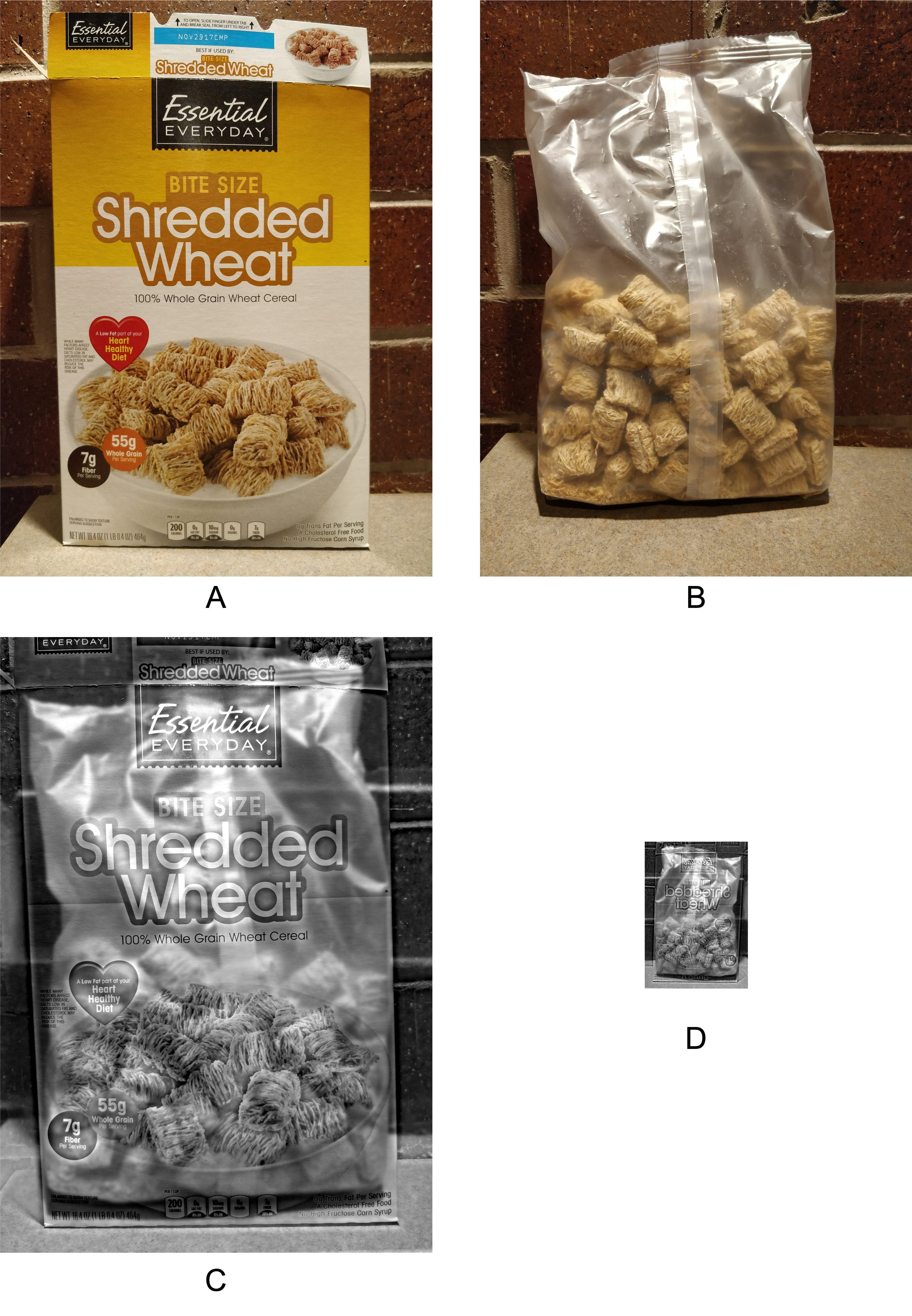
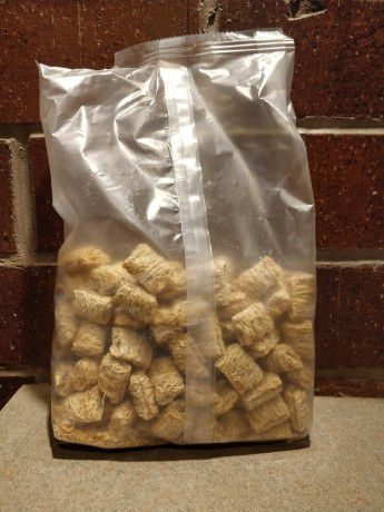
Hybrid images are static images with two interpretations, which changes as a function of the viewing distance. Consider the example below.
Figures A and B are the input images of a cereal box and its contents respectively. Figures C and D are the same hybrid image displayed at
different resolutions. When we view the hybrid image at its normal size we see the cereal box and when we zoom out we see the bag of cereal.
Steps to create a hybrid image
For this task, you should first use the images A and B from the example above. In addition create two more hybrid images using input images of your own. Here are some guidelines for choosing good input images:
- Good input image pairs usually consist of one image of a smooth surface (eg. a picture of your face) and another of a textured surface (eg. a picture of a dog's face). This is because creating hybrid images combines the smooth (low-frequency) part of one image with the high-frequency part of another. Another good example pair would be an apple and orange.
- Edit the images to ensure that the objects are aligned.
- Ensure that there are no diffuse shadows on either image and the objects are clearly visible.
- Crop and align the images such that the objects and their edges are aligned. The alignment is important because it affects the perceptual grouping (read the paper for details). You are free to use any image editing tool for this and there is no need for code for this step.
- Read aligned input images and convert them to grayscale (you are only required to produce grayscale hybrid images for full credit; color is part of the extra credit).
- Apply a low-pass filter, i.e., a standard 2D Gaussian filter, on the first (smooth) image. You can use scipy function scipy.ndimage.gaussian_filter.
- Apply a high-pass filter on the second image. The paper suggests using an impulse (identity) filter minus a Gaussian filter for this operation.
- Use your intuition and trial and error to determine good values of σ for the high-pass and low-pass filters. One of the σ's should always be higher than the other (which one?), but the optimal values can vary from image to image.
- Add or average the tranformed images to create the hybrid image.
Extra Credit
- Try to use color images as input to the hybrid images task and analyze the results. To merge colored images, you will have to apply the filters on each of the three channels separately.
- Try to come up with interesting failure cases of hybrid images and possible reasons for failure.
- Create Gaussian and Laplacian pyramids similar to Fig. 7 in the paper to visualize the process of hybridizing images.
Part 2: Scale-space blob detection
The goal of Part 2 of the assignment is to implement a Laplacian blob detector as discussed in the this lecture.
Algorithm outline
- Generate a Laplacian of Gaussian filter.
- Build a Laplacian scale space, starting with some initial scale and
going for n iterations:
- Filter image with scale-normalized Laplacian at current scale.
- Save square of Laplacian response for current level of scale space.
- Increase scale by a factor k.
- Perform nonmaximum suppression in scale space.
- Display resulting circles at their characteristic scales.
Test images
Here are four images to test your code, and sample output images for your reference. Keep in mind, though, that your output may look different depending on your threshold, range of scales, and other implementation details. In addition to the images provided, also run your code on at least four images of your own choosing.Detailed instructions
- You need the following Python libraries: numpy, scipy, scikit-image, matplotlib.
- Don't forget to convert images to grayscale (use convert('L') if you are using PIL)
and rescale the intensities to between 0 and 1 (simply divide them by 255 should do the trick).
- For creating the Laplacian filter, use the scipy.ndimage.filters.gaussian_laplace function.
Pay careful attention to setting
the right filter mask size. Hint: Should the filter width be odd or even?
- It is relatively inefficient to repeatedly filter
the image with a kernel of increasing size. Instead of increasing
the kernel size by a factor of k, you should downsample the image by a factor
1/k. In that case, you will have to upsample the result or do some
interpolation in order to find maxima in scale space. For full credit,
you should turn in both implementations: one that increases filter size,
and one that downsamples the image. In your report, list the running times
for both versions of the algorithm and discuss differences (if any) in the
detector output. For timing, use time.time().
Hint 1: think about whether you still need scale normalization when you downsample the image instead of increasing the scale of the filter.
Hint 2: Use skimage.transform.resize to help preserve the intensity values of the array.
- You have to choose the initial scale, the factor k by which the scale
is multiplied each time, and the number of levels in the scale space.
I typically set the initial scale to 2, and use 10 to 15 levels in the
scale pyramid. The multiplication factor should depend on the largest scale
at which you want regions to be detected.
- You may want to use a three-dimensional array to represent your
scale space. It would be declared as follows:
scale_space = numpy.empty((h,w,n)) # [h,w] - dimensions of image, n - number of levels in scale space
Then scale_space[:,:,i] would give you the i-th level of the scale space. Alternatively, if you are storing different levels of the scale pyramid at different resolutions, you may want to use an NumPy object array, where each "slot" can accommodate a different data type or a matrix of different dimensions. Here is how you would use it:
scale_space = numpy.empty(n, dtype=object) # creates an object array with n "slots"
scale_space[i] = my_matrix # store a matrix at level i - To perform nonmaximum suppression in scale space, you should first do
nonmaximum suppression in each 2D slice separately. For this, you may find
functions scipy.ndimage.filters.rank_filter or scipy.ndimage.filters.generic_filter useful.
Play around with these functions, and try to find the one that works the fastest.
To extract the final nonzero values (corresponding to detected regions),
you may want to use the numpy.clip function.
- You also have to set a threshold on the squared Laplacian response above
which to report region detections. You should
play around with different values and choose one you like best. To extract values above the threshold,
you could use the numpy.where function.
- To display the detected regions as circles, you can use
this function
(or feel free to search for a suitable Python function or write your own).
Hint: Don't forget that there is a multiplication factor
that relates the scale at which a region is detected to the radius of the
circle that most closely "approximates" the region.
Extra Credit
-
Implement the difference-of-Gaussian pyramid as
mentioned in class and described in David Lowe's paper.
Compare the results and the running time to the direct Laplacian implementation.
- Implement the affine adaptation step to turn circular blobs into
ellipses as shown in the lecture (just one iteration is sufficient).
The selection of the correct window function is essential here. You should use
a Gaussian window that is a factor of 1.5 or 2 larger than the characteristic scale
of the blob. Note that the lecture slides show how to find the relative shape of the
second moment ellipse, but not the absolute scale (i.e., the axis lengths are defined
up to some arbitrary constant multiplier). A good choice for the absolute
scale is to set the sum of the major and minor axis half-lengths to the
diameter of the corresponding Laplacian circle. To display the resulting
ellipses, you should modify the circle-drawing function or look for a better
function in the matplotlib documentation or on the Internet.
- The Laplacian has a strong response not only at blobs, but also along edges. However, recall from the class lecture that edge points are not "repeatable". So, implement an additional thresholding step that computes the Harris response at each detected Laplacian region and rejects the regions that have only one dominant gradient orientation (i.e., regions along edges). If you have implemented the affine adaptation step, these would be the regions whose characteristic ellipses are close to being degenerate (i.e., one of the eigenvalues is close to zero). Show both "before" and "after" detection results.
Grading Checklist
As before, you must turn in both your report and your code. Your report will be graded based on the following items:Part 1:
- The original, filtered, and hybrid images for all 3 examples (i.e., 1 provided and 2 pairs of your own).
- Explanation of any implementation choices such as library functions or changes to speed up computation.
- For each example, give the two σ values you used. Explain how you arrived at these values. Discuss how successful your examples are or any interesting observations you have made.
- Optional: discussion and results of any bonus items you have implemented.
Part 2:
- The output of your circle detector on all the images (four provided and four of your own choice), together with running times for both the "efficient" and the "inefficient" implementation.
- An explanation of any "interesting" implementation choices that you made.
- An explanation of parameter values you have tried and which ones you found to be optimal.
- Discussion and results of any extensions or bonus features you have implemented.
Submission Instructions:
You must upload five files to Compass 2g.- Your code in two Python notebooks. The filenames should be netid_mp2_part1_code.ipynb or netid_mp2_part2_code.ipynb.
- Your ipython notebooks with output cells converted to PDF format. The filenames should be netid_mp2_part1_output.pdf and netid_mp2_part2_output.pdf.
- A single report for both parts in PDF format. The filename should be netid_mp2_report.pdf.
Don't forget to hit "Submit" after uploading your files, otherwise we will not receive your submission.
Please refer to course policies on collaborations, late submission, and extension requests.
Useful Python Links
- Scipy Gaussian Filter
- OpenCV Filter2D
- Sample Harris detector using scikit-image.
- Blob detection on Wikipedia.
- D. Lowe, "Distinctive image features from scale-invariant keypoints," International Journal of Computer Vision, 60 (2), pp. 91-110, 2004. This paper contains details about efficient implementation of a Difference-of-Gaussians scale space.
- T. Lindeberg, "Feature detection with automatic scale selection," International Journal of Computer Vision 30 (2), pp. 77-116, 1998. This is advanced reading for those of you who are really interested in the gory mathematical details.